1. Abstract
This study shows that the reliance on CNN (Convolutional Neural Network) is unnecessary for computer vision. Vit (Vision Transformer) attains excellent results when pre-trained on large amounts of data and transferred to multiple mid-sized or small image recognition benchmarks.
2. Introduction
In NLP (Natural Language Processing), Transformer architectures have become the dominant model, achieving strong results through large-scale pre-training and fine-tuning. However, CNN remain the standard in vision tasks, and although some works integrate self-attention into CNNs, these models have yet to fully replace convolutions.
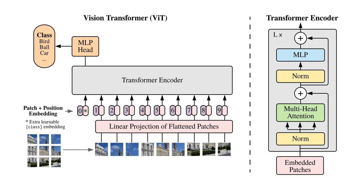
Inspired by the success of Transformers in NLP, this study proposes to apply a standard Transformer directly to images with minimal modifications: an image is split into patches, linearly embedded, and processed as a sequence of tokens — analogous to words in NLP. The study train the model on image classification in supervised fashion.
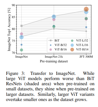
When trained on mid-sized datasets such as ImageNet, Transformers perform slightly worse than comparably sized ResNets. However, when trained on very large datasets (14M–300M images), large-scale training compensates for this, and the ViT achieves or surpasses state-of-the-art CNNs on several benchmarks, requiring substantially fewer computational resources.
3. Method
Model overview
3.1 Vit
Step 1: Since the standard transformer receives 1D sequence as input, we reshape the image $x∈R^{H×W×C}$ into a sequence of flattened 2D patches $x_p∈R^{N×(P^2⋅C)}$, where
$H×W$: resolution of the image $C$:number of channels $P^2$:resolution of each image patch $N=HW/P^2$:resulting number of patches, also serves as the input sequence length for the transformer
Step 2: Since the transformer uses constant latent vector size $D$ through all of its layers, we flatten the patches and map to $D$ dimensions with a trainable linear projection.
linear projection equation: $z^0 = [x_{\text{class}}; x^1_p E; x^2_p E; \dots; x^N_p E] + E_{\text{pos}} , E ∈ R^{(P^2·C)×D}, E_{\text{pos}} ∈ R^{(N+1)×D}$
Step 3: Step 3: Transformer Encoder and OutputThe embedded patches are passed through a series of $L$ Transformer Encoder layers. Each layer consists of two main sub-blocks: Multi-Head Self-Attention (MSA) and a Multi-Layer Perceptron (MLP).
- LayerNorm (LN) is applied before every block, and residual connections are applied after every block.
- The MLP contains two layers with a GELU non-linearity.
- The final output $y$ is the representation of the
[class]token, which is used for image classification.Encoder equations:$$z’{\ell} = \text{MSA}(\text{LN}(z{\ell-1})) + z_{\ell-1}, \quad \ell = 1 \dots L$$$$z_{\ell} = \text{MLP}(\text{LN}(z’{\ell})) + z’{\ell}, \quad \ell = 1 \dots L$$Final Output:$$y = \text{LN}(z_L^0)$$(where $z_L^0$ is the first token of the last layer’s output, representing the whole image features for classification.)
3.2 Inductive bias
Compared to CNNs, Vision Transformers (ViT) possess much less image-specific inductive bias. In CNNs, properties such as locality, two-dimensional neighborhood structure, and translation equivariance are hard-coded into the model architecture from the first layer to the last.
In ViT, however, these characteristics are handled differently:
- Locality & 2D Structure: Only the MLP layers contain local and translationally equivariant properties, while the self-attention layers allow for global information interaction.
- 2D Structure Initialization: ViT only utilizes the 2D structure of the image at the very beginning of the process when cutting the image into patches.
- Position Embeddings: At initialization, position embeddings carry no 2D spatial information; all spatial relationships between patches must be learned by the model from the data.
- Resolution Adjustments: The 2D spatial structure is only explicitly utilized again during fine-tuning when the image resolution changes, requiring adjustment of the position embeddings.
3.3 Hybrid Architecture
In addition to using raw image patches, the authors proposed a Hybrid Model that combines CNNs with Transformers.
In this design:
- Feature Extraction: A CNN (such as ResNet) is first used to extract the feature maps of the image.
- Patch Embedding: The resulting CNN feature maps are then divided into patches and fed into the Transformer.
- Flexible Patch Size: The patch size can be as small as $1 \times 1$, meaning each spatial location of the CNN feature map is flattened into a sequence for linear projection.
Key takeaway: The input sequence for the Transformer does not necessarily have to come from raw image patches; it can also be derived from high-level features extracted by a CNN to benefit from global understanding.
4. Experiments
4.1 Setup
- Datasets: The study explores model scalability using the ILSVRC-2012 ImageNet dataset (1.3M images), its superset ImageNet-21k (14M images), and the proprietary JFT dataset (303M high-resolution images).
- Benchmarks: Models are evaluated across several tasks, including ImageNet (standard and cleaned-up ReaL labels), CIFAR-10/100, Oxford-IIIT Pets, and Oxford Flowers-102.
- Baseline Models: For comparison, the researchers use ResNet (BiT), utilizing Group Normalization and standardized convolutions instead of Batch Normalization.
- Hybrid Architecture: In hybrids, intermediate feature maps from a CNN (like ResNet) are fed into the Transformer with a patch size as small as $1 \times 1$ “pixel”.
- Evaluation Metrics: Performance is reported via fine-tuning accuracy on downstream datasets or few-shot accuracy obtained by solving a regularized least-squares regression problem.
4.2 Model Variants
ViT configurations are based on those used for BERT to maintain consistency.
| Model | Layers | Hidden size $D$ | MLP size | Heads | Params |
|---|---|---|---|---|---|
| ViT-Base | 12 | 768 | 3072 | 12 | 86M |
| ViT-Large | 24 | 1024 | 4096 | 16 | 307M |
| ViT-Huge | 32 | 1280 | 5120 | 16 | 632M |
- Notation: A brief notation like ViT-L/16 denotes the “Large” variant with a $16 \times 16$ input patch size.
- Complexity: The Transformer’s sequence length is inversely proportional to the square of the patch size; therefore, models with smaller patch sizes are more computationally expensive.
4.3 Training
- Optimizer: All models, including ResNets, are trained using Adam.
- Hyperparameters: Settings include $\beta_1 = 0.9$, $\beta_2 = 0.999$, and a large batch size of 4096.
- Regularization: A high weight decay of 0.1 is applied, which was found useful for the transfer of all models.
- Learning Rate: A linear learning rate warmup and decay are utilized.
5. Conclution
5.1 Comparison to State of the Art
Performance Analysis
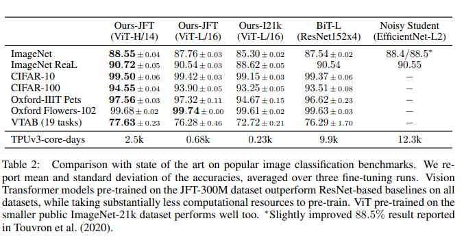
- Superior Accuracy: ViT models (especially ViT-H/14) outperform state-of-the-art CNNs like BiT and Noisy Student across multiple benchmarks including ImageNet and VTAB.
- Pre-training Impact: While JFT-300M provides the best results, ViT pre-trained on ImageNet-21k also shows competitive performance.
Computational Efficiency
- Resource Advantage: A major highlight of ViT is its training efficiency. ViT-L/16 outperforms BiT-L while requiring significantly fewer computational resources (0.68k vs 9.9k TPUv3-core-days).
- Efficiency Scaling: Even the largest ViT-H/14 model (2.5k core-days) is substantially cheaper to train than the leading CNN baselines.
5.2 Pre-training Dataset Size Analysis
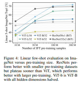
The Necessity of Large Data
- Small Datasets: ViT overfits significantly on ImageNet (1.3M) and underperforms compared to ResNets (BiT).
- Scalability: ViT’s performance scales much better than CNNs. Larger ViT variants only show their true benefits when trained on datasets like JFT-300M.
Inductive Bias vs. Learning from Data
- Findings: ResNets perform better with small pre-training samples due to convolutional inductive bias.
- Shift Point: Once the dataset exceeds 90M+ images, ViT starts to outperform ResNets of comparable computational cost.
Compute Efficiency
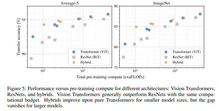
- Cost-Effectiveness: ViT provides a better performance-to-compute ratio than ResNets across most experimental settings.
- Hybrid Models: Useful for smaller computational budgets, but the advantage vanishes as the model and dataset size increase.