2.2 The Variational Bound (Variational Inference)
The authors proposed to use a neural network to find an encoder function $q_\psi(x)$ to approximate the true posterior $p_{\theta^}(z|x)$, and a decoder function to approximate the true generative model $p_{\theta^}(x|z)$ (data distribution)
For any probability density function of the observed data $x$, we can maximize the corresponding log-likelihood with our input data. The log-likelihood of our input data can be decomposed into:
$\text{log}p(x)=\text{log}p(x)\int_zq(z|x)dz$
$=\int_zq(z|x)\text{log}p(x)dz$
$=\int_zq(z|x)\text{log}(\frac{p(x, z)}{p(z|x)})dz$
$=\int_zq(z|x)\text{log}(\frac{p(x, z)}{q(z|x)}\frac{q(z|x)}{p(z|x)})dz$
$=\int_zq(z|x)\text{log}(\frac{p(x, z)}{q(z|x)})dz+\int_zq(z|x)\text{log}(\frac{q(z|x)}{p(z|x)})dz$
, where $q(z|x)$ is the posterior distribution of $z$ given the input data $x$.
Let the first term on the right-hand side be:
$L_b=\int_zq(z|x)\text{log}(\frac{p(x, z)}{q(z|x)})dz$
, and the second term on the right hand side would be:
$D_{KL}(q(z|x);||;p(z|x)) = \int_zq(z|x)\text{log}\frac{q(z|x)}{p(z|x)}dz$
Since Kullback–Leibler divergence (KL divergence) is always $\geq 0$ (proof):
$\text{log}p(x)=L_b+D_{KL}(q(z|x);||;p(z|x))\geq L_b+0=L_b$
To maximize the log-likelihood of $p(x)$, we try to maximize the lower bound $L_b$, this is also known as the evidence lower bound (ELBO) of log-likelihood of $p(x)$.
Let’s further decompose $L_b$:
$L_b=\int_zq(z|x)\text{log}(\frac{p(x, z)}{q(z|x)})dz$
$=\int_zq(z|x)\text{log}(\frac{p(x| z)p(z)}{q(z|x)})dz$
$=\int_zq(z|x)\text{log}p(x| z)dz+\int_zq(z|x)\text{log}(\frac{p(z)}{q(z|x)})dz$
$=\int_zq(z|x)\text{log}p(x| z)dz-D_{KL}(q(z|x);||;p(z))$
Kullback–Leibler divergence
Definition
$D_{KL}(q(x);||;p(x)) = \int_xq(x)\text{log}\frac{q(x)}{p(x)}dx$
Interpretation
- The measurement of distinguishing the two distribution $p$ and $q$ based on the observed data $x$ (if $x$ is drawn from $p$, what is the likelihood ratio of $p$ and $q$)
2.3 The SGVB estimator and AEVB algorithm (Reparameterization)
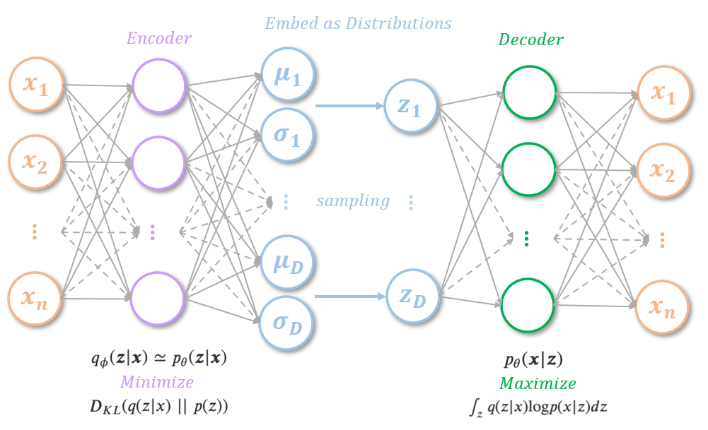
However, the parameters for the encoder and the decoder couldn’t be optimized using gradient ascend as there’s a sampling process dependent on the parameters in forward propagation. The authors proposed a reparameterization trick to address this. Instead of sampling from a Gaussian distribution $N(\mu, \sigma^2)$ that dependent on $\mu$ and $\sigma$, the reparameterization trick sample a Gaussian noise, and use the following equation to approximate the sampling while decoupling the parameters and the sampling process:
$z_i=\mu_i+\sigma_i\varepsilon_i$
, where $\varepsilon\sim N(0, 1)$. The neural network then becomes:
Decomposition of the Loss Function
$L_b=\int_zq(z|x)\text{log}p(x| z)dz+\frac{1}{2}\sum\limits_{j=1}^D[1+\log(\sigma_j)-(\sigma_j)^2-(\mu_j)^2]$
The first term of the ELBO is often referred to as the reconstruction loss. For the decoder to correctly decode the distribution into different data points in the feature space. The embedding distribution for different data points needs to be separated.
There are two straightforward ways of achieving this:
- The first way is to embed the data into distributions with minimal standard deviation. However, this makes variational autoencoder degenerates into autoencoder and the network will not be able to generate data points from unseen distributions in the latent space.
- The second way is to scatter the mean of the distribution of each data point across the entire latent space, however, the model couldn’t learn the relevant representation from the data point as well.
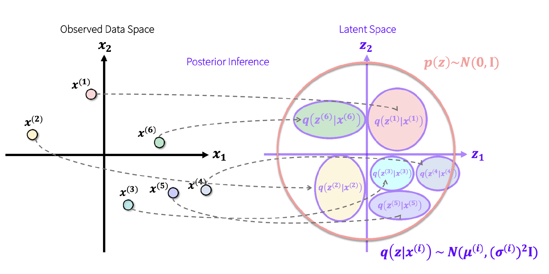
To prevent this, the KL divergence term can be thought of as a regularization. Assuming the marginal distribution of $p(z)$ follows a standard Gaussian distribution and $q(z|x)$ follows a multivariate Gaussian distribution, the second term of the ELBO can be solved by:
$-D_{KL}(q(z|x);||;p(z))=\frac{1}{2}\sum\limits_{j=1}^D[1+\log(\sigma_j)-(\sigma_j)^2-(\mu_j)^2]$
,where $D$ is the number of latent dimensions, $\mu_j$ and $\sigma_j$ is the mean and standard deviation from $j$-th components in the multivariate Gaussian distribution $q(z|x)$.
- The KL divergence punishes distributions with large mean values to prevent the distribution from scattering across the entire embedding space and the term $1+\log(\sigma_j)-(\sigma_j)^2$ prevent the variance to diminish.
- In order to maximize the likelihood, the term $\mu_j$ needs to be as close to 1 as possible.
This regularized the latent representation so that the data is constrained with a prior distribution $p(z)\sim N(0, I)$.
$1+\log(\sigma_j)-(\sigma_j)^2$ in the KL divergence
$1+\log(\sigma_j)-(\sigma_j)^2$ in the KL divergence
The encoding process (recognition network) can be conceptually visualized as:
The generative process (decoder network) can be conceptually visualized as:
image.png
The Variational Autoencoder
image.png
5 Experiment Data
MNIST
- ~70,000 hand written digit images with 28 x 28 x 1 features (for each pixel, only stores 0 or 1)
from Wikipedia “MNIST database”
from Wikipedia “MNIST database”
Frey Face
- ~1,965 images of Brendan Frey’s face (from sequential frames of video) with 28 x 20 x 1 features (for each pixel, store values between 0 - 1)
from Elvis Dohmatob
from Elvis Dohmatob
Some Experiments
Train a variational autoencoder on MNIST, the latent distributions (and its corresponding generated images)
image.png
References
- Auto-Encoding Variational Bayes. Kingma et al., ICLR 2014.
- Deep Learning DS-GA 1008, New York University. Spring 2018.