
Paper: https://arxiv.org/abs/1312.5602
This paper is mainly talking about the first deep learning model to successfully learn control policies directly from high-dimensional sensory input using reinforcement learning. The model is a convolution neural network, trained with a variant of Q-learning, whose input is raw pixels and whose output is a value function estimating future rewards.
Reinforcement Learning (quick review)
Reinforcement learning (RL) is a subfield of machine learning where an agent learns to make sequential decisions by interacting with an environment to achieve a specific goal. The agent receives rewards or penalties for its actions, and its objective is to find a strategy (called a policy) that maximizes the cumulative reward over time.
1. Introduction
Issues for using deep learning in reinforcement learning
- It have to learn from a scalar reward signal that is frequenly sparse, noisy and delayed.
- Deep learning algorithms assume the data samples to be independent, while in reinforcement learning one typically encounters sequences of highly correlated states.
- In RL, the data distibution changes as the algorithm learns new behaviors, which can be problematic for deep learning methods that assume a fixed underlying distribution.
Overcoming way:
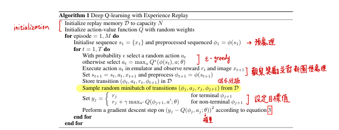
Use convolution neural network. The network is trained with a variant of the Q-learning algorithm, with stochastic gradient descent to update the weights. To alleviate the problems of correlate data and non-stationary distributions, we use an experience replay mechanism, which randomly samples previous transitions, and thereby smooths the training distribution over many past behaviors.
Convolutional Neural Network: Tackle high dimensional image/video inputs
Experience Replay Mechanism : Tackle high correlated data and non-stationary distributions. There will be a buffer (mermory) to store the history using a tuple, (sₜ , aₜ , rₜ , sₜ₊₁), and the model will randomly sample some of the history to train, so that the model can be train less correlated and avoid overfitting.
Example: If at sₜ the action got a super high reward, and sₜ₊₁ is a really similar situation and with the same aciton, but it got a bad reward, the model will get confused. In order to smooth that, we use replay mechanism to train a small batch of the past which might include sₜ, so that the model will have a better training.
2. Background
We consider tasks in which an agent interacts with an environment ε, in this case the Atari emulator, in a sequence of actions, observations and rewards. At each time-step the agent selects an action at from the set of legal game actions, A = {1,…,K}.
Since the agent only observes images of the current screen, the task is partially observed and many emulator states are perceptually aliased, i.e. it is impossible to fully understand the current situation from only the current screen xₜ. We therefore consider sequences of actions and observations, sₜ = {x₁, a₁, x₂,…, aₜ₋₁, xₜ}, and learn game strategies that depend upon these sequences. ( all sequence are assumed to terminate in a finite number of time-steps )
Reward, Rₜ: $$ R_t = \sum_{t’=t}^{T} \gamma^{t’-t} r_{t’} $$
$\gamma$ is the discount for the reward of each time-step, which means the more near present the more important the reward is. $$ Q^*(s, a) = \max_{\pi} \mathbb{E}[R_t | s_t = s, a_t = a, \pi] $$ This equation is saying the best outcome from (s, a)
- Q: Aciton-value function
- Q: optimal action-value funciton
- $\pi$: policy mapping sequence to actions (or distribution over acitons)
$$ Q^(s, a) = \mathbb{E}{s’ \sim \mathcal{E}} \left[ r + \gamma \max{a’} Q^(s’, a’) \middle| s, a \right] $$
The Q* equation can also written in this form. $\mathbb{E}_{s’ \sim \mathcal{E}}[\dots | s, a]$: The reason it is Expected value is that the enviroment is stochastic.
Such value iteration algorithms converge to the optimal action value function, Qᵢ→Q* as i→∞. In practice, this basic approach is totally impractical, because the action-value function is estimated separately for each sequence, without any generalisation. Instead, it is common to use a function approximator to estimate the action-value function, Q(s, a, θ)≈Q*(s, a). θ is the weight of the Q-network. A network that can be trained by minimising a sequence of loss function $L_i(\theta_i)$ that changes at each iteration i.
$$ L_i (\theta_i) = \mathbb{E}_{s,a \sim \rho(\cdot)} \left[ \left( y_i - Q(s, a; \theta_i) \right)^2 \right] $$
$$ y_i = \mathbb{E}{s’ \sim \mathcal{E}} \left[ r + \gamma \max{a’} Q(s’, a’; \theta_{i-1}) \middle| s, a \right] $$ $\rho(s, a)$ is a probability distibution over sequences s and action a that we refer to as the behavior distribution.
The objective of the loss function $L_i(\theta_i)$ is to minimize the squared difference between these two terms:$$\text{Loss} = (\text{Target Q-value} - \text{Current Q Prediction})^2$$By minimizing this loss, we are forcing the output of the Current Q-Network ($Q(s, a; \theta_i)$) to converge towards the stable Target Q-value ($y_i$), which is derived from the Bellman Optimality principle.
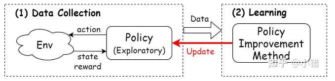
The aciton is using ε-greedy, which means it won’t always take the maxQ(s, a), it will try random action with probability of ε, in order to try new unexplored and possible better option.
3. Deep Reinforcement Learning
Our goal is to connect a reinforcement learning algorithm to a deep neural network which operates directly on RGB images and efficiently process training data by using stochastic gradient updates. We store the agent’s experiences at each time-step, eₜ = (sₜ , aₜ , rₜ , sₜ₊₁) in a data-set D = e₁,…, eₙ , pooled over many episodes into a replay memory. During the inner loop of the algorithm, we apply Q-learning updates, or minibatch updates, to samples of experience, e∼D, drawn at random from the pool of stored samples. After performing experience replay, the agent selects and executes an action according to an-greedy policy.
This approach has several advantages over standard online Q-learning:
- greater data efficiiency
- break the correlation
- avoid the divergence in the parameters
4. Experiments
We have performed experiments on seven popular ATARI games– Beam Rider, Breakout, Enduro, Pong, Q*bert, Seaquest, Space Invaders. Since the scale of scores varies greatly from game to game, we fixed all positive rewards to be 1 and all negative rewards to be -1, leaving 0 rewards unchanged. Clipping the rewards in this manner limits the scale of the error derivatives and makes it easier to use the same learning rate across multiple games.
In these experiments, we used the RMSProp algorithm with minibatches of size 32. The behavior policy during training was-greedy with annealed linearly from 1 to 0.1 over the first million frames, and fixed at 01 thereafter. We trained for a total of 10 million frames and used a replay memory of one million most recent frames.
we also use a simple frame-skipping technique. More precisely, the agent sees and selects actions on every kth frame instead of every frame, and its last action is repeated on skipped frames.
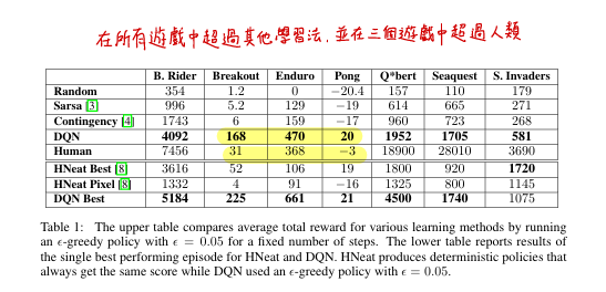
Conclusion: This paper introduced a new deep learning model for reinforcement learning, and demonstrated its ability to master difficult control policies for Atari 2600 computer games, using only raw pixels as input. We also presented a variant of online Q-learning that combines stochastic minibatch up dates with experience replay memory to ease the training of deep networks for RL. Our approach gave state-of-the-art results in six of the seven games it was tested on, with no adjustment of the architecture or hyperparameters.